Detecting my cats with Detectron2
24-01-2020In this post I'll show how train a model with Detectron2 with a custom dataset and then apply it detect my cats in a picture or video.
Table of content
- Install Detectron2
- Create your own dataset
- Steps to annotate an image
- Training process
- Data loader
- Inference
- References
Install Detectron2
I use the docker version of Detectron2 that installs all the requirements in a few steps:
1. Take the required files, Dockerfile, Dockerfile-circleci, docker-compose.yml from https://github.com/facebookresearch/detectron2/tree/master/docker
2. Create and run the container with the command:
docker-compose run --volume=/local/path/to/save/your/files:/tmp:rw detectron2
The installed version of Pillow package is 7.0.0, this could fail when you try to train your model showing an error similiar to:
                                from PIL import Image, ImageOps, ImageEnhance, PILLOW_VERSION

                            ImportError: cannot import name 'PILLOW_VERSION'
The solution is to downgrade the version to 6.2.2:
pip install --user Pillow==6.2.2
Check the installation guide to install Detectron2 using other methods.
Create your own dataset
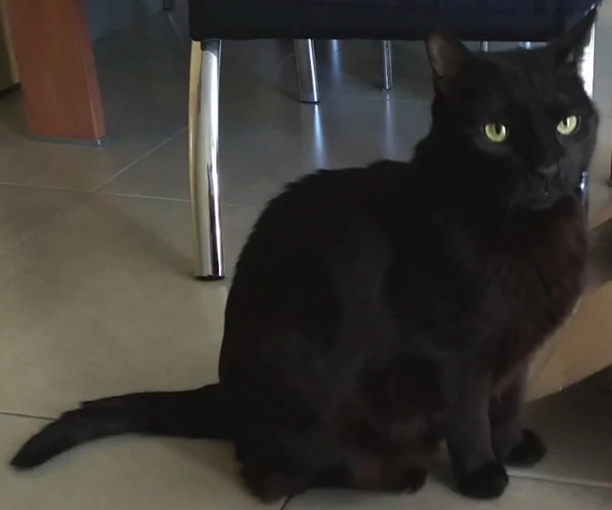
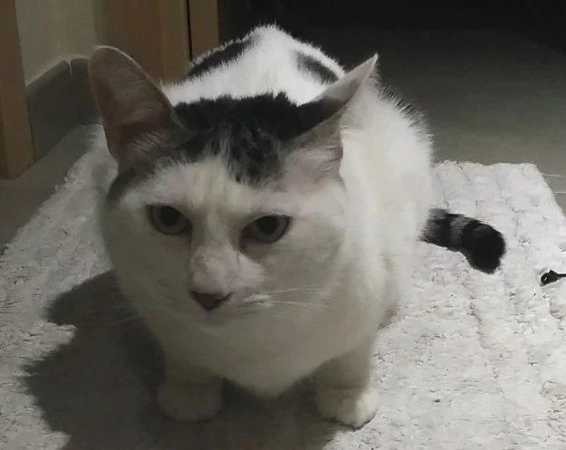
The first (and most tedious) step is to annotate the images. For this examples I will use a set of images of my cats, Blacky and Niche:
Steps to annotate an image
- The instructions below are for VIA tool, if you are using a different tool, then jump to the next section.
- Follow this process twice, once for training images, another for validation images.
Before start to annotating the images you must create a region attribute named Class, you can change the name if you want, in order to choose which region your are drawing.
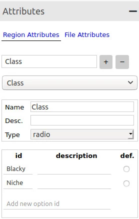
Looking the image above, follow these steps:
1. Expand the Attributes panel.
2. Type the attribute name Class on textbox and click on plus symbol.
3. Change the Type of the attribute from text to radio.
4. Write all classes available for the dataset, Blacky and Niche in my case, in the id field.
Next, the basics steps to annotate the images:
1. Add the images to the project clicking on the Add Files button in the Project panel.
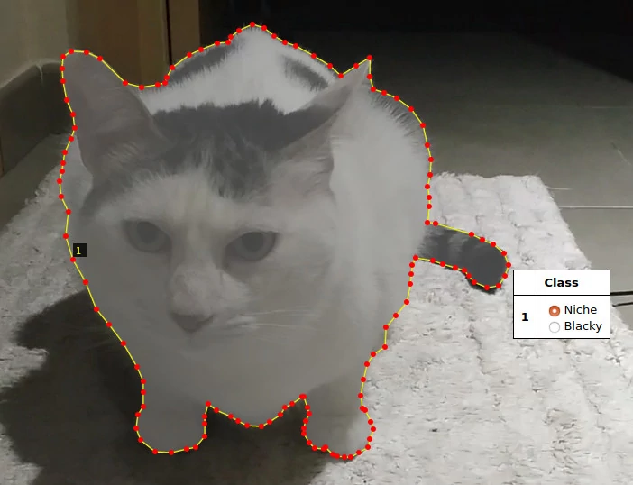
2. Select one image and start drawing the region using the Poligon region shape.
3. To apply the changes press Enter and the region will be saved.
4. Click outside of the region, click again on the region and select the class you are annotating.
The json file will contains a section by image similar to this one:
                            "frame80.jpg214814": {

                              "filename": "frame80.jpg",

                              "size": 214814,

                              "regions": [

                                {

                                  "shape_attributes": {

                                    "name": "polygon",

                                    "all_points_x": [

                                      1096,

                                      1016,

                                      947,

                                      ...

                                    ],

                                    "all_points_y": [

                                      116,

                                      191,

                                      231,

                                      ...

                                    ]

                                  },

                                  "region_attributes": {

                                    Class": "Blacky"

                                  }

                                }

                              ],

                              "file_attributes": {}

                            }

                            ...
Training process
Before to start to explain the code, let me show the folder structure in order to have an idea of where are the code, the data and all this stuff.
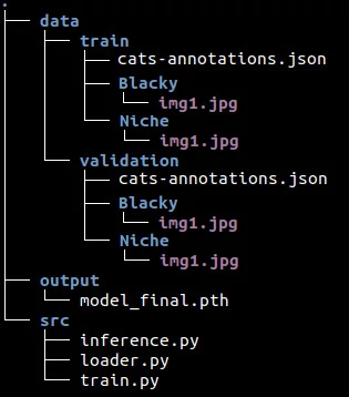
The data folder contains two folders, train and validation, which contain one folder per class (of course, there are more than one image in the class folder). Also, the train and validation folders have its respective annotation files. The src folder contains the code sepated in different files.
Ok, now we are ready to write the code. First things first, we need to import the functions required from detectron2.
                            # train.py


                            import os


                            from detectron2.data import MetadataCatalog, DatasetCatalog

                            from detectron2.config import get_cfg

                            from detectron2 import model_zoo

                            from detectron2.engine import DefaultTrainer

                            from loader import get_data_dicts
Next, we'll register both datasets, train and validation, and indicate the name of the classes that we are using.
                            for d in ["train", "val"]:

                              DatasetCatalog.register("cats_" + d, lambda d=d: get_data_dicts("../data/" + d))

                              MetadataCatalog.get("cats_" + d).set(thing_classes=["Blacky", "Niche"])


                            cats_metadata = MetadataCatalog.get("cats_train")
The DatasetCatalog.register function expects two parameters, the name of the dataset, and the function to get the data.
With MetadataCatalog we specify which classes are present in the dataset using the attribute thing_classes. To know more about the metadata check the documentation.
Now let's configure the model:
                            cfg = get_cfg()

                            cfg.merge_from_file(model_zoo.get_config_file("COCO-InstanceSegmentation/mask_rcnn_R_50_FPN_3x.yaml"))

                            cfg.DATASETS.TRAIN = ("cats_train",)

                            cfg.DATASETS.TEST = ()

                            cfg.DATALOADER.NUM_WORKERS = 4

                            cfg.MODEL.WEIGHTS = "detectron2://COCO-InstanceSegmentation/mask_rcnn_R_50_FPN_3x/137849600/model_final_f10217.pkl"

                            cfg.SOLVER.IMS_PER_BATCH = 2

                            cfg.SOLVER.BASE_LR = 0.00025

                            cfg.SOLVER.MAX_ITER = 700

                            cfg.MODEL.ROI_HEADS.BATCH_SIZE_PER_IMAGE = 128

                            cfg.MODEL.ROI_HEADS.NUM_CLASSES = 2
- get_cfg(): returns an instance of CfgNode class that allow us to modify the configuration of the model.
- cfg.merge_from_file: we use this to apply the original configuration from mask_rcnn_R_50_FPN_3x model to our configuration.
- cfg.DATASETS.TRAIN: This is the list of dataset names for training. Important to note the comma at the end.
- cfg.DATASETS.TEST: This remains empty for the training purposes.
- cfg.DATALOADER.NUM_WORKERS: Number of data loading threads.
- cfg.MODEL.WEIGHTS: Pick the weights from mask_rcnn_R_50_FPN_3x model.
- cfg.SOLVER.IMS_PER_BATCH: Number of images per batch.
- cfg.SOLVER.BASE_LR: Learning rate.
- cfg.SOLVER.MAX_ITER: Total iterations (Detectron2 don't use epochs).
- cfg.MODEL.ROI_HEADS.BATCH_SIZE_PER_IMAGE: Indicate the number of ROI's (Region of Interest) per training minibatch.
- cfg.MODEL.ROI_HEADS.NUM_CLASSES: Number of classes.
Basically what we are doing here is to get configuration from an existing model, mask_rcnn_R_50_FPN_3x, then we overwrite some of the values like learning rate, iterations, etc...
Check the documentation about the configuration to know all available options that you can change.
And finally it's time to call the training process:
                            os.makedirs(cfg.OUTPUT_DIR, exist_ok=True)

                            trainer = DefaultTrainer(cfg)

                            trainer.resume_or_load(resume=False)

                            trainer.train()
Data loader
Now it's time to implement the function to let Detectron2 know how to obtain the data from the dataset that we registered before with:
DatasetCatalog.register("cats_" + d, lambda d=d: get_data_dicts("../data/" + d))
The code of loader.py is pretty similar to the function shown in the Colab notebook
                            # loader.py


                            def get_data_dicts(img_dir):

                              classes = ["Blacky", "Niche"]


                              json_file = os.path.join(img_dir, "cats-annotations.json")

                              with open(json_file) as f:

                                imgs_anns = json.load(f)


                              dataset_dicts = []

                              for idx, v in enumerate(imgs_anns.values()):

                                record = {}


                                if "regions" not in v: continue


                                # Extract info from regions

                                annos = v["regions"]

                                objs = []


                                for anno in annos:

                                  shape_attr = anno["shape_attributes"]

                                  px = shape_attr["all_points_x"]

                                  py = shape_attr["all_points_y"]

                                  poly = [(x + 0.5, y + 0.5) for x, y in zip(px, py)]

                                  poly = [p for x in poly for p in x]


                                  region_attr = anno["region_attributes"]

                                  current_class = region_attr["Class"]

                                  obj = {

                                    "bbox": [np.min(px), np.min(py), np.max(px), np.max(py)],

                                    "bbox_mode": BoxMode.XYXY_ABS,

                                    "segmentation": [poly],

                                    "category_id": classes.index(current_class),

                                    "iscrowd": 0

                                  }

                                  objs.append(obj)


                                record["annotations"] = objs


                                # Get info of the image

                                filename = os.path.join(img_dir, current_class, v["filename"])

                                height, width = cv2.imread(filename).shape[:2]


                                record["file_name"] = filename

                                record["image_id"] = idx

                                record["height"] = height

                                record["width"] = width


                                dataset_dicts.append(record)

                              return dataset_dicts
The function loops through all annotations in the json file and extract the information related with the region, category, etc... of the image.
The annotation itself is represented by the dictionary obj that contains some specific keys:
- bbox: list of 4 numbers representing the bounding box of the instance.
- bbox_mode: the format of the bbox.
- category_id: number that represents the category label.
- iscrowd: 0 or 1. Whether the instance is labeled as COCO's format.
Also, some extra information is saved in the record dictionary:
- file_name: the fullpath of the image.
- image_id: a unique id to identify the image.
- height: self explanatory.
- width: self explanatory.
To know more about of the dictionary check the documentation.
Inference
It's time to do some predictions and we start with the imports:
                            # inference.py


                            import os

                            import random

                            import cv2


                            from detectron2.config import get_cfg

                            from detectron2 import model_zoo

                            from detectron2.engine import DefaultPredictor

                            from detectron2.utils.visualizer import Visualizer, ColorMode

                            from detectron2.data import MetadataCatalog

                            from loader import get_data_dicts
For inference we use a few different functions: DefaultPredictor, Visualizer and ColorMode.
Next, we configure the model as we did on the training process, then create the predictor:
                            classes = ["Blacky", "Niche"]


                            cfg = get_cfg()

                            cfg.merge_from_file(model_zoo.get_config_file("COCO-InstanceSegmentation/mask_rcnn_R_50_FPN_3x.yaml"))

                            cfg.DATASETS.TEST = ("cats_val",)

                            cfg.MODEL.WEIGHTS = os.path.join(cfg.OUTPUT_DIR, "model_final.pth")

                            cfg.MODEL.ROI_HEADS.NUM_CLASSES = 2

                            cfg.MODEL.ROI_HEADS.SCORE_THRESH_TEST = 0.7


                            predictor = DefaultPredictor(cfg)
This configuration is similar to the configuration we used in the training but this time the WEIGHTS come from our trained model model_final.pth.
                            dataset_dicts = get_data_dicts("../data/validation")


                            for idx, d in enumerate(random.sample(dataset_dicts, 3)):

                              im = cv2.imread(d["file_name"])

                              outputs = predictor(im)


                              v = Visualizer(im[:, :, ::-1],

                                metadata = MetadataCatalog.get("cats_val").set(

                                  thing_classes=classes,

                                  thing_colors=[(177, 205, 223), (223, 205, 177)]),

                                scale = 0.8,

                                instance_mode = ColorMode.IMAGE_BW

                              )


                              pred_class = (outputs['instances'].pred_classes).detach()[0]

                              pred_score = (outputs['instances'].scores).detach()[0]


                              print(f"File: {d['file_name']}")

                              print(f"--> Class: {classes[pred_class]}, {pred_score * 100:.2f}%")


                              # Save image predictions

                              v = v.draw_instance_predictions(outputs["instances"].to("cpu"))

                              image_name = f"inference_{idx}.jpg"

                              cv2.imwrite(image_name, v.get_image()[:, :, ::-1])
To make the predicitions we use 3 random images from the validation dataset.
The predictor receive the image in format BGR, the same format that cv2 returns when reads the image. Once we have the predictions then we create and configure the Visualizer that we'll use to show the regions predicted over the original image.
The Visualizer accepts as the first parameter the original image but this time in RGB format, that's why we have to reverse the array that cv2 returns when reads the image.
The second parameter is the metadata, which in this case consists of the name of the classes, Blacky and Niche, and the colors applied to the regions of each class.
The ColorMode.IMAGE_BW value is used to remove the color of unsegmented pixels (the pixels that don't belong to the predicted region).
At the end we apply the regions predicted over the original image with v.draw_instance_predictions(outputs["instances"].to("cpu"))
In this case I save the image on disk because I don't have access to XServer from inside Docker, so OpenCV cannot open any window to show the image. In case we worked from our local system we could use:
                            v = v.draw_instance_predictions(outputs["instances"].to("cpu"))

                            cv2.imshow(v.get_image()[:, :, ::-1])
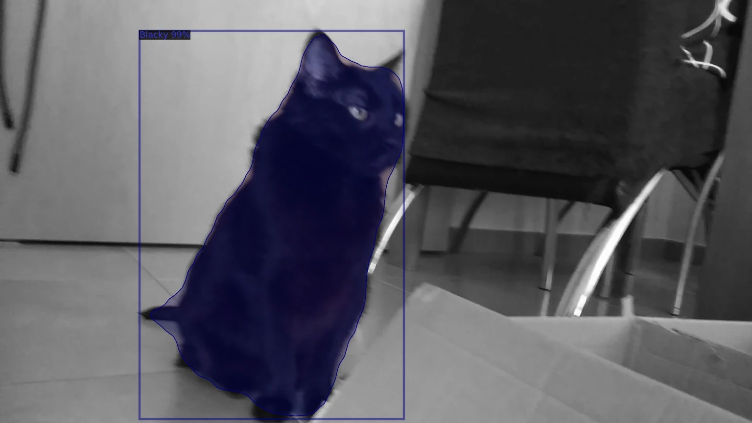
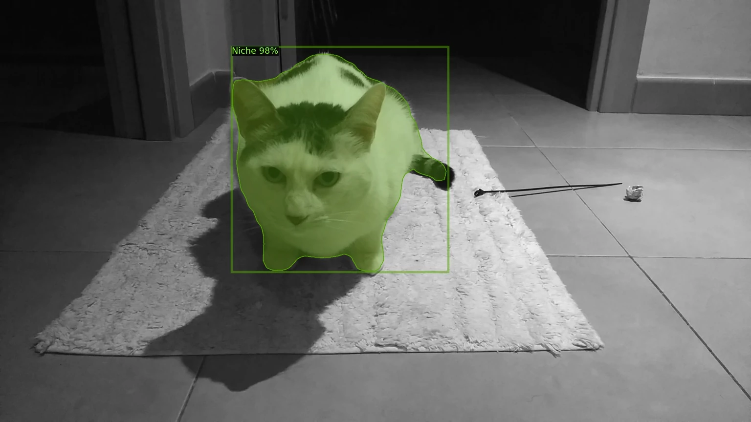
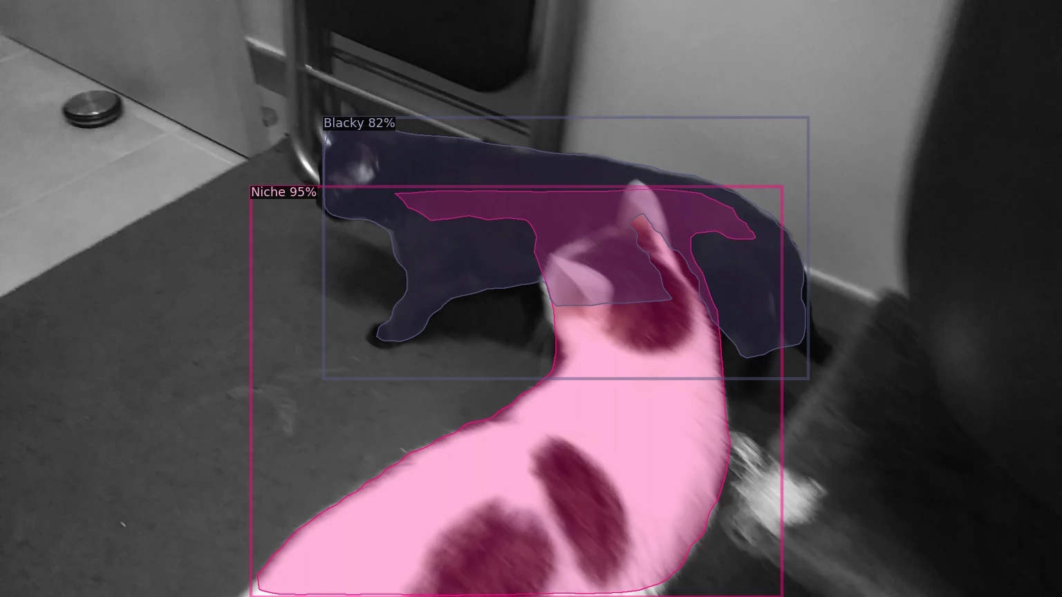
Check the test.py file in the repository to know how to make inference in a video. Spoiler alert: predicting every frame xD.
COMMENTS